Homework 3
Getting your assignment: You can find template code for your submission here at this GitHub Classroom link. All of the code you write you should go in hw3.Rmd, and please knit the Markdown file in your completed submission.
Introduction
An important problem in inferential learning is that the data available are almost always too sparse to unambiguously pick out the true hypothesis (see e.g. Quine, 1960). Human learners, however, appear to cope with this problem just fine, converging on a small set of possible hypothesis from very little data. In machine learning, this is known as few-shot learning, and is a real challenge for modern learning systems. One hypothesis for what helps human learners is that have a strong prior on the kinds of hypotheses that are likely and relevant, which makes the search problem much easier.
In this assignment, you’ll be working with a simple problem designed to demonstrate this phenomenon, and building a model that learns in a human-like way. The number game, developed by Josh Tenenbaum (2000), demonstrates the power of strong sampling for inductive inference. The key insight is that the probability that data is generated by a hypothesized process is proportional to the size of the set of possible data that the hypothesis could generate.
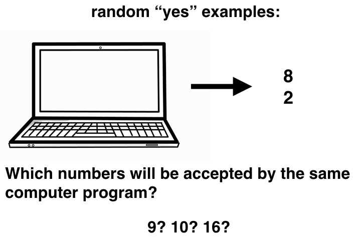
In the number game, you get as input one or more numbers between 1 and 100 generated by a computer program according to an unknown rule. Your job is to determine the most likely rule, or to make predictions about which numbers the program will generate next.
Modeling the number game
To figure out what hypothesis the computer is generating samples from, you can use Bayesian inference. To do this, you will use Bayes Rule to infer the posterior probability for each hypothesis:
\[ P\left(H \vert D\right) \propto P\left(D \vert H\right)P\left(H\right)\]
To specify the model, you need to specify a prior probability (\(P\left(H\right)\)) for each hypothesis, and a likelihood function that specified how probable the observed data are under that hypothesis (\(P\left(D \vert H\right)\)).
Prior: Following Tenenbaum (2000), we’ll say that hypotheses can be of two kinds: Mathematical and Interval. We’ll say that aprior, there is a \(\lambda\) probability that the true hypothesis is in the set of Mathemtical hypotheses, and a (1-\(\lambda\)) probability that the true hypothesis is in the set of Interval Hypotheses
Likelihood: If we assume that the every number consistent with a particular hypothesis is equally likely to be generated by the machine, then if every number in \(D\) is in \(H\), the likelihood that set of numbers \(D\) is generated by the hypothesis \(H\) is the probability of choosing \(\lvert D \rvert\) numbers at random from the set of \(\lvert H \rvert\) numbers (\(\frac{1}{\lvert H \rvert \choose \lvert D \rvert}\)). You can compute this in R using the choose function. Otherwise, \(H\) cannot generate \(D\) and the likelihood is 0.
The candidate hypotheses
Your first goal is to write all of the candidate hypotheses that your model will consider. You don’t need to exhaustively include all of the hypotheses in the original Tenenbaum (2000) model, just the following
Mathematical hypotheses:
even numbers
odd numbers
square numbers
cube numbers
prime numbers
multiples of any number \(n\), \(\left(3 \leq n \leq 12\right)\)
powers of any number \(n\), \(\left(2 \leq n \leq 10\right)\)
Interval hypotheses:
decades (\(\left\{1-10,\; 10-20, \;\ldots \right\}\))
any range \(1 \leq n \leq 100, n \leq m \leq 100, \left\{n-m\right\}\)
One nice way of representing these hypotheses as tibbles with two columns: name which gives a human-readable description of the hypothesis, and set which is a list of all of the numbers 1—100 consistent with that hypothesis. You’ll first. write a function that generates each of these. For the multiple-set hypotheses (e.g. multiples of any number), you can make the function generate a multi-row tibble where each row is one of the sub-hypotheses.
Problem 1: Define all of the hypotheses for the number game. You’re welcome to use the stubs I have provided in the template. (3 points).
Now that you have each of the individual hypotheses, you can put them all together. A nice representation for this is one big tibble that has a row for all of the hypotheses you’ve generated. You’ll find the bind_rows function to be helpful here.
The last detail is that you want to be able to assign a prior probability appropriately to each of these hypotheses. Remember, all of the mathematical hypothesis together should have prior probability \(\lambda\), and the interval hypotheses should make up the remainder of the prior (\(1 - \lambda\)). You’ll want to divy up this probability equally within those respective sets.
Problem 2: Write the function make_all_hypotheses which takes in a value for the parameter \(\lambda\) and construct the full tibble of hypotheses. It should have four columns: name, set, type (mathematical or interval), and prior which have a value of each of all of the possible hypotheses. Hint: There should be 5,084 total (1 point).
Modeling Inference
Now that you have all of your hypotheses, you need to write the likelihood function. And finally to compute the posterior probability of each hypothesis.
Problem 3: Write the function compute_likelihood which takes in a set of numbers consistent with a hypothesis \(H\) , and a set of input numbers \(D\), and which returns the likelihood of generating that input set from that hypothesized number set (\(P\left(D \vert H\right)\)) (1 point).
Problem 4: Write the function best_hypotheses which takes in a tibble of hypotheses (\(H\)), a set of input numbers \(D\), an optional number of hypotheses \(n\), and returns a tibble with the top \(n\) hypotheses for the data according to the posterior probability (\(P\left(H \vert D\right)\)) as well as their corresponding posterior probability. You might find it helpful not to return every row of the original hypotheses tibble, but only their type (mathematical or interval), name, and posterior (2 points).
Inferring hypotheses
Now you are ready to test the model! Using the default \(\lambda\) value of \(\frac{4}{5}\), you will get the top 5 best hypotheses for each of the following sets of data \(D\):
\(2\)
\(2, 4, 8\)
\(15, 22\)
\(1, 2, 3, 4, 6\)
Problem 5: Print out the top 5 best hypotheses according to the model for each of these values. Does the model predict what you think it should? Were there any surprises? (2 points)
Problem 6: Try changing the value of \(\lambda\) to something smaller, like \(\frac{1}{5}\). What effect does this have on the model’s predictions for the examples above? (1 point)
Predicting the next number.
Now you will implement the final part of the model: Prediction about whether the computer is likely to generate a new number \(d'\) having observed all of the previous examples \(D\). To do this, you will use Bayesian model averaging. Instead of committing to the best hypothesis after observing \(D\), you will average together all of the hypotheses, weighing them by the posterior probability of them being true after observing \(D\).
\[ P\left(d'\right) = \sum_{h \in H}P\left(d' | h\right)P\left(h | D\right)\]
You’ll just need to write one new function predict_value which will take in a tibble of hypotheses, a set of previously observed numbers, and a new target number. It should return the posterior probability of observing that number according to the formula above. You shouldn’t need any new helper functions here!
To check whether it works correctly, try these examples using the default value for \(\lambda\):
\(D = 2, \;d' = 12\)
\(D = 2, 4, 8, \;d' = 12\)
\(D = 15, 22 \; d' = 21\)
\(D = 15, 22 \; d' = 50\)