Homework 4
Getting your assignment: You can find template code for your submission here at this GitHub Classroom link. All of the code you write you should go in hw4.Rmd, and please knit the Markdown file in your completed submission.
Introduction
In the last decade, we have seen an explosion of impressive results in Machine Learning, producing models that match and even sometimes outperform humans on challenging tasks. A non-trivial part of the challenge in developing these models is not in specifying how they should solve the problems they are developed solve, but in figuring out how to actually derive predictions from these models.
Earlier this semester, we read a paper from Charles Kemp, And Perfors, and Josh Tenebaum that shows how overhypotheses like the shape bias can be understood through the lens of rational analysis. Because the model does not have an analytic solution, A sizeable chunk of the article describes approximation methods that the authors use for for determining approximately what the model predicts.
The approach that Kemp et al. use, and that is a mainstay in modern Bayesian approaches, is technique called Markov chain Monte Carlo (MCMC). Markov chain Monte Carlo is a method for approximating samples from a complex Distribution by drawing samples from other simpler distributions and reweighing or combining them together.
In this assignment, you will implement the Metropolis Algorithm, an MCMC algorithm in the sequential sampling family. In this family of algorithms, samples are drawn from a simple Proposal distribution and then either Accepted (if they have high probability under the target distribution), or Rejected in favor of keep the current sample.
The Metropolis Algorithm
Metropolis is a simple sequential sampling scheme for drawing samples from a target distribution \(P\left(x\right)\) by using a density function \(f\left(x\right)\) that is proportional to \(P\)– i.e., that can give the relative probability of two different samples \(x\) and \(x'\).
The algorithm works by starting a chain at some arbitrary point \(x_0\). Then, in each iteration \(t\), a new sample \(x1\) by modifying the previous sample \(x_{t}\) according to a proposal distribution \(g\left(x'|x_{t}\right)\). The critical requirement is that \(g\) is a symmetric distribution \(g\left(x'|x\right) = g\left(x|x'\right)\).
For your simulation, you should use a simple Normal distribution centered at the previous sample \(g\left(x'|x\right) \sim \text{Normal}\left(x, \sigma\right)\).
You then run the algorithm for some number of iterations, e.g. 1000, at each iteration performing the following steps:
Propose a new sample \(x'\) by drawing from \(g\left(x'|x_{t}\right)\)
Compute the acceptance ratio \(\alpha = \frac{f\left(x'\right)}{f\left(x\right)}\)
Sample \(u \sim \text{Uniform}\left(0,1\right)\).
If \(u \leq \alpha\), accept the proposed sample (\(x_{t+1} = x'\)).
Otherwise, reject the proposed sample and keep the previous sample (\(x_{t+1} = x_{t}\)).
Sampling from an Exponential Distribution
Exponential distributions are a common distribution in models of cognition, for example they are sometimes used to model forgetting in memory. The Exponential distribution has one parameter \(\lambda\) which defines the rate of decay (or forgetting).
If \(x \sim \text{Exponential}\left(\lambda\right)\), \(P\left(x\right) = \lambda e^{-\lambda x}\).
R actually can draw samples from an Exponential distribution. For example, here are 1000 samples from \(\text{Exponential}\left(3\right)\)
samples <- tibble(sample = 1:1000, value = rexp(1000, rate = 3))

ggplot(samples, aes(x = value)) +
  geom_histogram(fill = "white", color = "black")b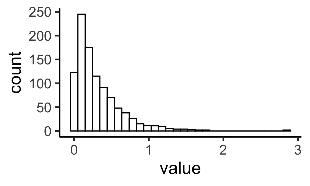
But let’s see how can draw samples from an exponential distribution using Metropolis-Hastings samples instead.
You will need to do 4 things:
Define the Exponential target distribution \(f(x)\) using the Exponential definition above.
Define the proposal distribution \(g(x'|x)\)
Define and Metropolis sequential sampling algorithm
Run the Algorithm for some number of iterations and plot the results.
Problem 1: Implement the Exponential probability density function. This function should take in a value \(x\) and a parameter \(\lambda\) and return the probability of sampling the value \(x\) from the Exponential distribution with parameter \(\lambda\) (see above, 1 point).
Problem 2: Implement a Gaussian proposal function. This should take in a current value \(x\), a parameter sigma which defines how wide the proposal distribution is. It should return a new proposed sample \(x'\) (1 point).
One thing you might notice is that the Metropolis samples won’t look like Exponential samples right away. Here is a plot of \(f(x)\) for 1000 samples from Metropolis:
ggplot(output, aes(x = iteration, y = f)) +
  geom_line()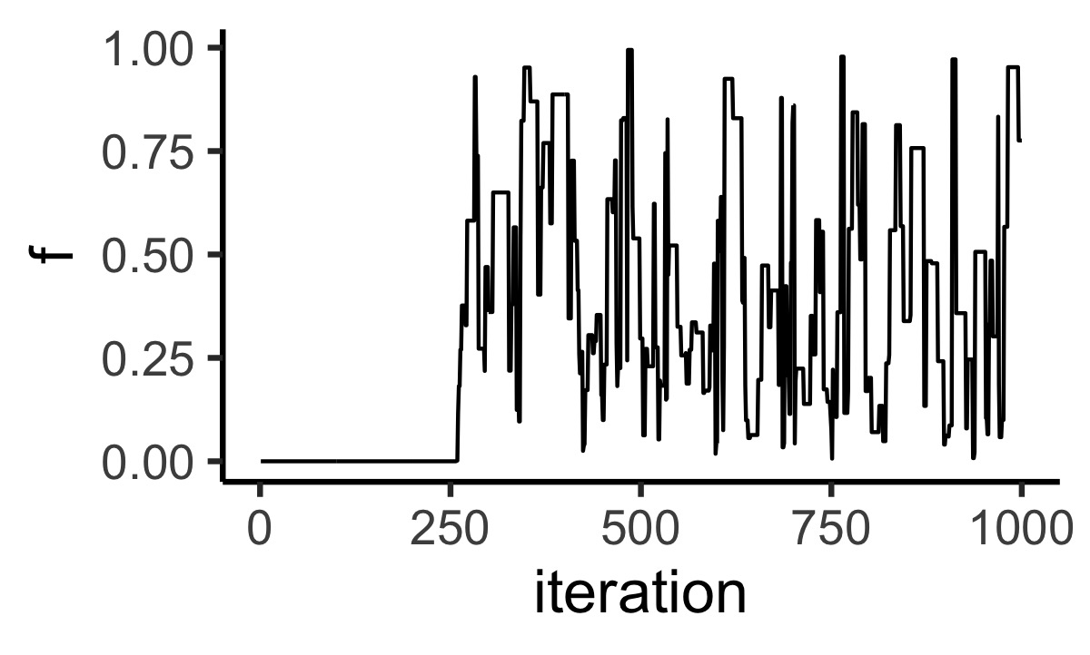
You can see that first several hundred samples, every sample has low probability under the target distribution. This happens when the starting point of the chain is far away from the area of high density in the target distribution. For this reason, it is common to discard some of the initial samples–a process called burn in. You may find this helpful in future simulations.
Problem 3: Implement a Metropolis sampler for an Exponential distribution and use it draw 1000 samples from an Exponential distribution with \(\lambda=3\). Try \(\lambda=1\) as well. Do the distributions look different? You should use the two functions you just wrote for Problems 1 and 2. (2 points)
Sampling from a Dirichlet Distribution
The Dirichlet Distribution is a highly flexible distribution that is that can many different forms depending on its parameters. It often finds use in Cognitive models precisely when the goal is to learn about something than has unknown shape before learning starts (e.g. the probability of category membership given some set of features). It’s also not available in the R statistics library. You can sample from it using MCMC!
The Dirichlet distribution takes \(K \geq 2\) parameters (corresponding to separate dimensions) which are commonly represented as a vector \(\boldsymbol \alpha\). Each \(\alpha_{i} \geq 0\) is a concentration parameter which specifies how much of the probability mass of the function is concentrated on that dimension.
For a vector \(\boldsymbol x\),
\[ \text{Dirichlet}(\boldsymbol x) = \frac{1}{B\left(\boldsymbol\alpha\right)} \prod_{i=1}^{K}{x_{i}^{\alpha_{i} - 1}} \]
Where \(B\) is a normalizing constants: The \(Beta\) function
\[ \text{Beta}(\boldsymbol \alpha) = \frac{\prod_{i=1}^{K}{\Gamma\left(\alpha_{i}\right)}}{\Gamma\left(\sum_{i=1}^{K}\alpha_{i}\right)} \]
And \(\Gamma\) is the continuous generalization of the factorial (\(x!\)) function. You can call it in R with gamma(x)
You can use Metropolis to sample from the Dirichlet distribution in the same way you did for the Exponential distribution with one wrinkle: You need a different proposal distribution. The exponential distribution is defined over all positive real numbers, so you used Gaussian proposals and simply cut the distribution off when \(x < 0\). However, the Dirichlet distribution is defined only when the value on every dimension is between 0 and 1, and the sum of the values across the dimensions adds up to 1 (this is called a simplex). So if you try to make Gaussian proposals, almost every proposal will be rejected because the Dirichlet distribution will give probability 0 for it.
Instead, you can use a proposal function where you generate values from a uniform distribution between a small negative and small positive fraction, and this fraction to one dimension while subtracting it from the other. This will keep your \(x\)s in the desired range.
Problem 4: Implement the Beta function, the Dirichlet distribution probability function, and the Delta proposal function. The equations will be different from the functions above, but the process should be very similar (2 points).
Problem 5: Implement a Metropolis sampler for a Dirichlet distribution and use it draw samples from a Dirichlet distribution with \(\alpha = <.7,4>\). How many burn in samples do you need before the chain stabilizes? (2 points)
Inference via Markov Chain Monte Carlo
In addition to it’s utility in sampling from complex distributions, MCMC is a powerful tool for inference in these same distributions. If we have samples from a distribution with unknown parameters, we can use MCMC to infer the parameters that generated it (e.g. we can infer the category structure most likely to have produced the exemplars we observed).
In the final part of the assignment, you will use Metropolis to infer the unknown parameters of a Dirichlet distribution from a set of samples from it. To do this, we will leverage Bayes’ rule: \(P\left(H|D\right) \propto P\left(D|H\right)P(H)\). In the previous section, you used the likelihood function for a known Dirichlet distribution \(P(D|H)\) in order to draw samples from it. Now you will use that same likelihood function for inference. The intuition here is that the parameters that assign high probability to a given sample are more likely to have been the source of that sample.
In the previous sections, in each iteration you proposed a sample from the distribution and rejected it if it was not sufficiently likely. Now, you will propose hypothetical parameters for the distribution, and reject them if they do not make the sample sufficiently likely.
The homework template will provide you 100 samples from this unknown Dirichlet distribution and your job will be to recover the parameters that generated it. Think carefully about the proposal distribution you want to use here. Remember, each proposal will now move you around on the parameter space of the Dirichlet distribution–not the space of values produced by the Dirichlet.